A common question when transferring an established process from one facility to another is how to establish that the transferred process is performing equivalently to the original process. Sounds like it should be an easy question to answer – just produce some batches in the receiving facility and compare to the process from the donor facility. But how do we compare? What tools are available to show that the new process is equivalent to the old process?
Some investigators test equivalency with a significance test. An example of such a test is the two-sample t-test. In a two-sample t-test, two data samples are compared to determine the probability that the sample data would result if the true difference in means between the two processes was zero. For example, if the t-test yields a probability greater than the chosen significance level, we would conclude that there is insufficient evidence to reject the hypothesis that the means of two data are equal. On the other hand, a probability less than the chosen significance level indicates that there is enough evidence to reject the hypothesis that the means of two data sets are equal; i.e., conclude that the two data sets do not come from equivalent processes. In this case we would say that the two process means are not statistically equivalent.
But wait – while we may have answered the question as to whether the two process means are statistically equivalent, the question of practical importance is whether the two process means are close enough to satisfy CUSTOMER requirements; i.e., whether the two means are equivalent. Determining the maximum difference (specification) that can be tolerated, requires a solid understanding of what the “customer” of the process requires. Investigators must adopt the mindset that customer requirements are of paramount importance, since being more strict than the customer drives high cost and failing to meet customer requirements drives away customers. Thus, investigators should use equivalence tests (not significance tests) to establish equivalence.
Although we cannot demonstrate statistically that no difference exists between two independent populations (the sample size would be too large!), we can use statistics to show that the difference between two population means is less than some predefined limit. This is where the two, one-sided test or TOST comes in.
Proper application of the TOST or equivalence test, requires the investigator to account for the inherent variation of each process. For example, assuming the donor process is in control, capable and ready for equivalence testing, we would not want to set equivalence limits tighter than the confidence interval bounds established for the donor process. Doing so would in effect be holding the recipient process to a higher standard than the donor process. Equivalence limits should be no tighter than those effects or differences considered to have practical importance for process output quality. In general, if the investigator wishes to state equivalence with the confidence commensurate to the undertaking of a technology transfer, significant focus will have been placed on process characterization, measurement system analysis and experimental design, execution and analysis.
Figure 1 helps to visualize how two process averages are compared in an equivalency test. The sample data from each process is used to estimate the probability distribution of the average for each. The average estimate comes across as a distribution because doing so factors in the critical consideration of the sample variation (which approximates the variation of the process). To understand the important roll variance plays, consider that while the average of 120, 100 and 80 and the average of 160, 100 and 40 are each 100, the range of the second data set is 3 times that of the first. In practice, the probability distribution of the average estimate is calculated using the standard deviation of the sample.
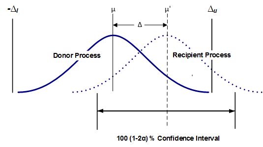
Figure 1 depicts as the observed difference and and as the maximum acceptable difference, together forming the equivalence interval of the two (2) process averages. Equivalence is established at the α significance level if a 100 (1–2α) % confidence interval for the difference between the two process averages is contained within the interval (, ). the confidence interval is (1–2α) and not the usual (1- α) because the TOST method is equivalent to performing two (individual) one-sided tests. Thus, using a 95% confidence interval for each individual one-sided test in effect yields a 90% confidence level when testing equivalence.
As with any statistical method, the degree of precision afforded by the test is dependent on the number of data available. The larger the sample size the less uncertainty we have in estimating the population parameters; e.g., mean and variance. Therefore, before conducting an equivalence test, an appropriate sample size for the test must be determined. The adequacy of a selected sample size is usually expressed in terms of test power. Test power is the probability that an effect of importance will be detected, should that effect exist. Power analysis is used to establish an appropriate sample size for a test given prior knowledge of the data variance and the effect or difference to be detected (see ProPharma blog “The Power to See Differences that Matter”, for more details on power and sample size).
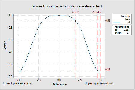
An example of a power curve generated for a 2-sample equivalence test is provided in Figure 2. In this example, given equivalence limits of -5 and 5 and a variance of 1, a sample size of 3 provides a test power of at least 0.91 for a ∆ of approximately 2 or less. In other words, when the real difference is 2, there is a 91% chance that a random sample of n=3 from each process will yield a result of equivalence (note: that is not to say that the estimated difference will be 2). But, for a ∆ of 4.6, the same sample size only provides a test power of 0.11 because n=3 samples with a standard deviation of 1.0 is (likely) insufficient to resolve a true mean difference 0.4 with the upper equivalence limit. Put another way, there is an almost 90% chance that the difference estimate (when the true mean is 4.6) will be greater than the upper equivalence limit. Not good odds for making the correct decision that the two means are equivalent.
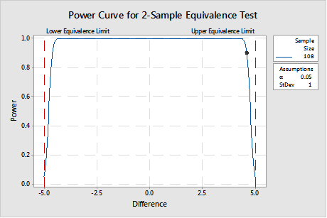
If in fact, if it is important to see a difference out to ±4.6 AND less than or equal to ± 5.0, then the sample size must be much larger, as shown in the power curve in Figure 3. This represents a significantly greater resource commitment, but it is worth it when product made in that range is safe and effective.1
The sample size must provide the correct balance between the time and money considerations pushing for a smaller sample size and the investment necessary to develop the process knowledge required to meet customer requirements.
After choosing an appropriate sample size (i.e., one providing adequate power at the equivalence bounds) for both donor and recipient processes and generating the required data, the TOST is conducted. If the confidence interval of the difference estimate is contained within the equivalence bounds, then equivalency between the two processes can be claimed. Conversely, if the confidence interval extends beyond one or both equivalence bounds, the claim of equivalence is rejected. If the claim of equivalence is rejected and experimental error is determined not to be a significant factor, the best option may be to accept the result and work to improve the donor process by, for example, shifting the mean and/or reducing the variation). However, the experimenter should also revisit/verify that the equivalence limits truly reflect the process requirements.
TOST equivalence tests overcome the limitations associated with traditional hypothesis tests when the goal is to demonstrate the equivalence of two data populations given stated equivalence bounds2. The TOST methodology allows the experimenter to discriminate between effects or differences that are merely statistically significant from those that are truly of practical importance.
Footnotes
- A rule of thumb for limiting sample size is that the smallest difference of interest is no less than one tenth of the specification range (in this case, the difference between the upper and lower equivalence limits). This is the same rule of thumb used for assessing/demonstrating measurement system adequacy.
- TOST is also recommended in USP general chapters <1033> and <1210> as a statistical tool for validating the accuracy and precision of analytical procedures.
References
- Hyde, Gary (2018). The Power to See Differences that Matter. Life Science Consulting. ProPharma Group, May 14, 2018.
- Hyde, Gary (2019). Innocent Until Proven Guilty: Hypothesis Test. Life Science Consulting. ProPharma Group, January 8, 2019.
- Limentani, Giselle B., Ringo, Moira C., Feng Ye, Bergquist Mandy L., McSorley, Ellen O. (2005). Beyond the t-Test: Statistical Equivalence Testing. Analytical Chemistry, 77 (11), 221 A– 226 A. DOI: 10.1021/ac053390m
- Walker, Esteban, PhD and Nowacki, Amy S., PhD (2010). Understanding Equivalence and Noninferiority Testing. Journal of General Internal Medicine, 26 (2), 192 – 196. DOI: 10.1007/s11606-010-1513-8
- Little, Thomas A. PhD (2015). Equivalence Testing for Comparability. BioPharm International, February 1, 2015. 28 (2).
- Lakens, Daniel (2017). Equivalence Tests: A Practical Primer for t Tests, Correlations, and Meta-Analyses. Social Psychological and Personality Science, 8 (4), 355-362. DOI: 10.1177/1948550617697177
- <1033> Biological Assay Validation. (2019). The United States pharmacopeia. The National formulary. Rockville, Md.: United States Pharmacopeial Convention, Inc.
- <1210> Statistical Tools for Procedure Validation. (2019). The United States Pharmacopeia. The National formulary. Rockville, Md.: United States Pharmacopeial Convention, Inc.
