Understanding Statistical Intervals: Part 3 - Tolerance Intervals

We saw in Part 1 of this series how a confidence interval can be calculated to define a range within which the true value of a statistical parameter such as a mean or standard deviation is likely to be located with a given confidence. In Part 2 we saw how a prediction interval can be calculated to define a region within which a single future observation or a multiple number of single future values is likely to be located with a given confidence. In this, the third and final statistical interval to be discussed, we will look at an interval to cover a specified proportion of a population distribution with a given confidence. This type of interval is called a tolerance interval and is closely related to measures of process capability.

Capability is usually expressed as the ratio of the specification range or tolerance for the measured characteristic to the observed variation associated with the characteristic. Larger ratios indicate a more capable process while smaller ratios indicate a less capable process. The capabilities of two different processes are depicted in Figure 1.

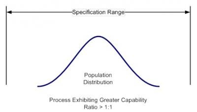
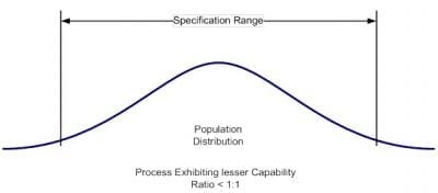
Looking at Figure 1, we can see that the distribution on the left exhibits good capability; the tail areas of this distribution are well within the specification range. The distribution on the right, on the other hand, exhibits poor capability; the tail areas of this distribution fall outside of specification range. Notice also that the capability of a process is determined not just by the location of the sample mean, but the tail areas of the distribution as well.

Because of physical, time or cost constraints, it is often impractical to inspect or test an entire production batch.  Instead, a small sample of a total population is inspected or tested and the data used to gauge how well the entire production batch conforms to specifications.

In traditional statistical process control, a significant number of data points are required in order to get a reasonably accurate estimate of process capability.  This is because capability is usually calculated to cover a fixed multiple of sample standard deviations (usually ±3 representing 99.73% of the data population). But this percentage only holds true for larger sample sizes; that is, greater than 50. As the sample size decreases, there is greater uncertainty in knowing the true location of the mean and the true magnitude of the population variance; therefore, the estimate of the range of values encompassing a given percentage of the population must necessarily increase to compensate.  Therefore, In order to maintain a reasonably accurate estimate of the capability of a process for smaller sample sizes, we need to adjust the number of multiple sample standard deviations used to define the region covering the desired proportion of the population distribution with a given confidence. A tolerance interval can be used for this purpose.

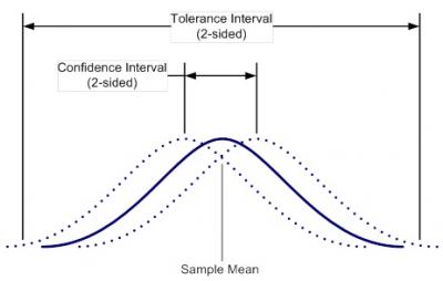
Figure 2 depicts a tolerance interval graphically. Notice in figure 2 that the interval range extends beyond the tail areas of the actual population distribution (solid line). This is because the tolerance interval must take into account the uncertainty of knowing the true location of the mean of the population distribution. This uncertainty is represented by the confidence level associated with the interval. The confidence level indicates the likelihood that the interval covers the desired proportion of the population.

Two-sided Tolerance intervals are calculated as:

Where x̄ is the sample mean; s is the sample standard deviation; and k₂ is a factor for a two-sided tolerance interval defining the number of sample standard deviations required to cover the desired proportion of the population.

Exact values of k₂ are tabularized in ISO 16269-6. These values of k₂ were calculated iteratively using a numerical integration process described by Garaj and Janiga in 2002. But this calculation, being very complex, is beyond the scope of this article.

However, in practice, a reasonable approximation of k₂ can be obtained using a formula originally proposed by Howe (1969) and later corrected by Guenther (1977):

Where:

n is the sample size;

Z_1-p/2    is the standard normal variate corresponding to one minus the proportion of the population to be covered divided by two.

is the critical value of the chi-square distribution with n-1 degrees of freedom surpassed with probability g, the statistical confidence.

For example, suppose we have assay data for ten randomly-selected containers of a drug product. We want to specify with a 95% level of confidence a range of assay values that will cover 99% of the data population in order to determine if the manufacturing process is capable. Let's assume for this example that the variation contributed by measurement method is insignificant with respect to the process variation. The assay data are given in Table 1.

Table 1. Assay data for ten randomly selected containers of a drug product

The validity of a tolerance interval is highly dependent on the underlying data distribution. In practice, data are assumed to be normally distributed; but we want to perform a test to determine if this assumption is valid.  This test can be performed graphically by creating a normal probability plot of the data. The y-axis on a normal probability plot represents the cumulative percentage of the data distribution and the x-axis represents the value of the measured characteristic. If the data are normally distributed, the data will fall fairly close to a straight line on the graph, the majority of the data being clustered near the 50th percentile.

The assumption of normality can also be tested by applying the Anderson- Darling test. The Anderson-Darling test yields a P-value that can be compared to the chosen significance level to determine whether or not the assumption of normality should be rejected. The significance level, a, chosen in this case is 0.05. Any value of P less than a indicates that there is sufficient evidence to reject the assumption of normality. A normal probability plot was created using Minitab® statistical software (figure 3).

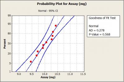
Figure 3 shows that the sample assay data closely follow a straight line. Also, the Anderson-Darling test returned a P-value much greater than 0.05; therefore, we would not reject the assumption that the data are normally distributed.

To calculate the tolerance interval we must first find the value of k2 corresponding to the desired confidence level, p=0.95, the desired proportion, p=0.95, and the degrees of freedom, n-1=9. We also need values for ^Z(1-p)/2 and X^2_y,n-1. The values for ^z(1-p

and

The extra "1-" term in the Excel formulas above is required because the Excel algorithms for the NORM.S.INV and CHISQ.INV functions utilize 1 minus the entered probability value. The extra "1-" term corrects the entered value so that the Excel functions yield the correct values.

In this example, the value of ^Z(1-p)/2 is 2.576 and, with 9 degrees of freedom, the value of X²_y,n-1 is 3.325. Plugging these values along with the sample size, n=10, into (2) yields:

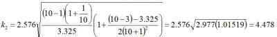
Knowing the value for k₂, the tolerance interval is then calculated, thus:

Now, if the target value of the process is 10mg and the specification limits are plus or minus 10% of the target value, the capability of the process based on a 99 % two-sided tolerance interval calculated with 95% confidence is:

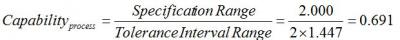
With a capability much less than 1, we can see that this process is not very capable.

There may also be situations where process capability is measured relative to a single-sided limit. These situations arise when a product characteristic need only meet a minimum specification limit or, remain below a maximum specification limit. In this case, we would want to make use of a one-sided tolerance interval. The calculation of an approximate k factor for a one-sided tolerance interval comes from a formula described by Natrella (1963):

(3)

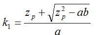
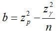
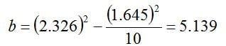
where

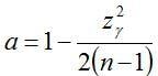
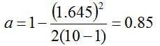
and

Suppose, for example, there is a maximum limit on the number of particles greater than a certain size contained within a liquid suspension drug product. 10 containers are randomly pulled from the finished product batch and tested for particle counts. The particle testing yields data presented in Table 2:

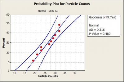
First, a normal probability plot was constructed for the data. Because the P-value is much greater than 0.05, there is no reason to reject the assumption that the data are normally distributed.

Next, we find the value of k₁ corresponding to the sample size, n=10, the desired confidence level, y=0.95, and the desired proportion, p=0.99. The values for Z_p and Z_y are calculated in Excel using the following NORM.S.INV Excel statistical function:

and

Plugging the values for

and the sample size, n=10, into equation 4 yields:

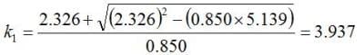
With the value for k₁ in hand, the tolerance interval is calculated as:

Thus, the upper 99% single-sided tolerance bound calculated with 95% confidence is 46. What this means is that for 95 out of 100 samples of size 10 taken from the same population, we would only expect 1% to have a particle count greater than 46.

If we were instead concerned with meeting a lower limit on particle counts rather than staying below a maximum value, we would simply subtract k₁ from the mean instead of adding as we did in the example above. In this case, the lower 99% single-sided tolerance bound calculated with 95% confidence is 6. If the lower specification limit in this case is 10, then the capability is:

Tolerance intervals are calculated using a variable multiple of sample standard deviations determined based not only on the desired confidence level and proportion of the population to be covered, but also the sample size available.  Thus, tolerance intervals yield reasonable estimations of process capability even with small data sets. Also, because tolerance intervals specify a region covering a proportion of the population, not just the uncertainty associated with a population parameter, tolerance intervals are the widest of the intervals. Tolerance intervals should be used when the capability of a process, that is, the ratio of a process specification to the population spread is the primary goal.

-Fred Wiles, Project Lead, ProPharma
January 16th, 2014

References

• NIST/SEMATECH e-Handbook of Statistical Methods, http://www.itl.nist.gov/div898/handbook/
• GARAJ, I and JANIGA, I. (2002). Two-sided tolerance limits of normal distribution for unknown mean and variability. Bratislava: Vydavatelstvo STU, p. 147.
• ISO 16269: 2005 Statistical interpretation of data - Part 6: Determination of statistical tolerance intervals.
• Howe, W. G. (1969). Two-sided tolerance limits for normal populations - some improvements. Journal of the American Statistical Association 64, pp. 610-620
• Natrella, M. G. (1963). Experimental Statistics, NBS Handbook 91, National Bureau of Standards, Washington, DC

Learn more about ProPharma's Technical Solutions services. Contact us to get in touch with Fred and our other subject matter experts for a customized Technical Solutions presentation.