August 15, 2013

August 15, 2013
Part 1 of this series discussed confidence intervals. Confidence intervals are the best known of the statistical intervals but they only bound regions associated with population parameters; i.e., the mean or standard deviation of a population. What if instead of the mean or standard deviation we are interested in individual observations from a population? For this we can make use of the prediction interval.
Prediction Intervals represent the uncertainty of predicting the value of a single future observation or a fixed number of multiple future observations from a population based on the distribution or scatter of a number of previous observations. Similar to the confidence interval, prediction intervals calculated from a single sample should not be interpreted to mean that a specified percentage of future observations will always be contained within the interval; rather a prediction interval should be interpreted to mean that when calculated for a number of successive samples from the same population, a prediction interval will contain a future observation a specified percentage of the time.
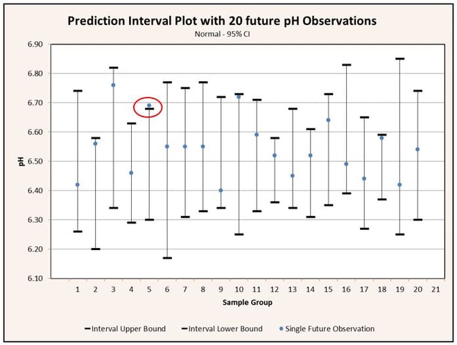
If we collect a sample of observations and calculate a 95% prediction interval based on that sample, there is a 95% probability that a future observation will be contained within the prediction interval. Conversely, there is also a 5% probability that the next observation will not be contained within the interval. If we collect 20 samples and calculate a prediction interval for each one, we can expect that 19 of the intervals calculated will contain a single future observation while 1 of the intervals calculated will not contain a single future observation. This interpretation of the prediction interval is depicted graphically in Figure 1.
Prediction intervals are most commonly used in regression statistics, but may also be used with normally distributed data. Calculation of a prediction interval for normally distributed data is much simpler than that required for regressed data, so we will start there.
The formula for a prediction interval is nearly identical to the formula used to calculate a confidence interval. Recall that the formula for a two-sided confidence interval is
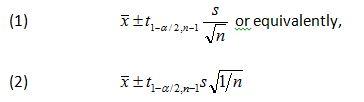
where x̄ is the sample average, s is the sample standard deviation, n is the sample size, 1-a is the desired confidence level, and t1-a/2:n-1 >is the 100(1-a/2) percentile of the student’s t distribution with n-1 degrees of freedom.
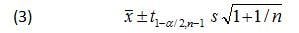
All that is needed for a formula to calculate a prediction interval is to add an extra term to account for the variability of a single observation about the mean. This variability is accounted for by adding 1 to the 1/n term under the square root symbol in Eq 2. Doing so yields the prediction interval formula for normally distributed data:
As an example, let’s again take a look at the pH example from Part I of this series. From the pH example we have the following data:
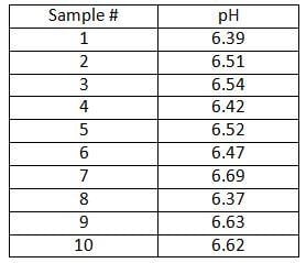
The analyst wants to know, based on the samples collected so far, the two-sided interval within which a single future pH observation is likely to lie with some level of confidence. The average pH, x, in this example is 6.52; the sample standard deviation, var, is 0.11. The confidence level chosen is 95% (a=0.05)
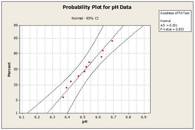
Unlike confidence intervals that are only concerned with the center of the population distribution, prediction intervals take into account the tails of the distribution as well as the center. As a result, prediction intervals have greater sensitivity to the assumption of normality than do confidence intervals and thus the assumption of normality should be tested prior to calculating a prediction interval. The normality assumption can be tested graphically and quantitatively using appropriate statistical software such as Minitab. For this example the analyst enters the data into Minitab and a normal probability plot is generated. The Normal Probability Plot is shown in Figure 2.
Looking at the probability plot we can see that all of the data fall within the 95% (1- a) Confidence Interval bands. Furthermore, the P-Value is much greater than the significance level of a = 0.05; therefore we would not reject the assumption that the data are normally distributed and can proceed with calculating the prediction interval.
To calculate the interval the analyst first finds the value t1-a/2,n-1 in a published table of critical values for the student’s t distribution at the chosen confidence level. In this example, t1-a/2,n-1 = t1-0.005/2,10-1 = 2.262.
Next, the values for t1-a/2,n-1 s, and n are entered into Eqn. 3 to yield the following prediction interval:

The interval in this case is 6.52 ± 0.26 or, 6.26 – 6.78. The interpretation of the interval is that if successive samples were pulled and tested from the same population; i.e., the same batch or same lot number, 95% of the intervals calculated for the individual sample sets will be expected to contain a single next future pH reading.
If, instead of a single future observation, the analyst wanted to calculate a two-sided prediction interval to include a multiple number of future observations, the analyst would simply modify the t in Eqn. 3. While exact methods exist for deriving the value for t for multiple future observations, in practice it is simpler to adjust the level of t by dividing the significance level, a, by the number of multiple future observations to be included in the prediction interval. This is done to maintain the desired significance level over the entire family of future observations. So, instead of finding the value for ta/2,n-1 we would find the value for ta/2k,n-1 where k is the number of future observations to be included in the prediction interval.
There are also situations where only a lower or an upper bound is of interest. Take, for example, an acceptance criterion that only requires a physical property of a material to meet or exceed a minimum value with no upper limit to the value of the physical property. In these cases the analyst would want to calculate a one-sided interval. To calculate a one-sided interval the analyst would simply remove the 2 from the divisor; thus ta/2,n-1 would become ta,n-1 and ta/2k,n-1 would become ta/k,n-1.
We turn now to the application of prediction intervals in linear regression statistics. In linear regression statistics, a prediction interval defines a range of values within which a response is likely to fall given a specified value of a predictor. Linear regressed data are by definition non-normally distributed. Normally distributed data are statistically independent of one another whereas regressed data are dependent on a predictor value; i.e., the value of Y is dependent on the value of X. Because of this dependency, prediction intervals applied to linear regression statistics are considerably more involved to calculate then are prediction intervals for normally distributed data.
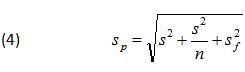
The uncertainty represented by a prediction interval includes not only the uncertainties (variation) associated with the population mean and the new observation, but the uncertainty associated with the regression parameters as well. Because the uncertainties associated with the population mean and new observation are independent of the observations used to fit the model the uncertainty estimates must be combined using root-sum-of-squares to yield the total uncertainty, Sp. Denoting the variation contributed by the regression parameters as Sf, the variation contributed by the estimate of the population mean as s/√n, and the variation contributed by the new measurement as s, the total variation, Sp, is defined as:
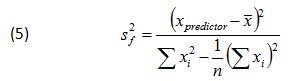
Where S2f is expressed in terms of the predictors using the following relationship:
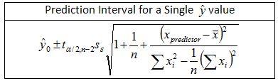
Adding Eqn. 5 to the other two terms under the square root in Eqn. 3, yields the two-sided prediction interval formula for the regressed response variable ŷ0
. The ‘hat’ over the y indicates that the variable is an estimate due to the uncertainty of the regression parameters and the subscripted 0 is an index number indicating that y is the first response variable estimated.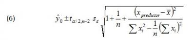
Evaluation of Eqn. 6 is best achieved using Analysis of Variance (ANOVA). Below is the sequence of steps that can be followed to calculate a prediction interval for a regressed response variable given a specified value of a predictor.
Calculate the slope and intercept of the regressed data
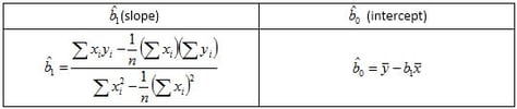
The equations in Step 3 represent the regression parameters; i.e., the slope and intercept defining the best fit line for the data. The prediction interval for the estimated response variable, ŷ0, must be evaluated at a specified x using the relationship ŷ0 = b̂1x+b̂0. The prediction interval then brackets the estimated response at the specified value of x.
Calculate the sum of squares and error terms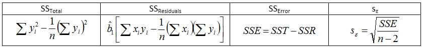
For example, suppose an analyst has collected raw data for a process and a linear relationship is suspected to exist between a predictor variable denoted by x and a response variable denoted by ŷ0. The analyst wants to know with 95% confidence the region in which a value for ŷ0. The raw data are presented below.
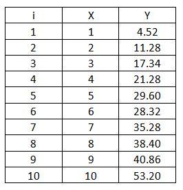
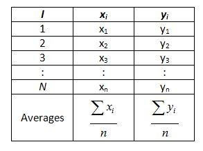
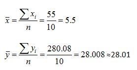
Following the ANOVA procedure outlined above, the analyst first calculates the mean of both the predictor variable, x, and the response variable,ŷ0.
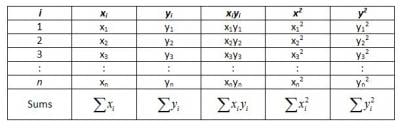
Next, the analyst prepares a table of sums.
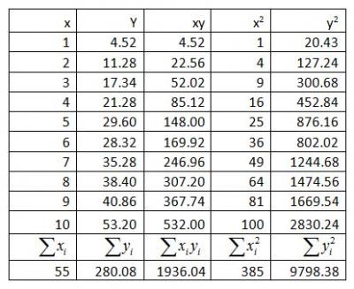
After completing the table of sums, the analyst proceeds to calculate the Slope (b̂1), Intercept (v̂0), Total Sum of Squares (SSTotal), Sum of Squares of the Residuals (SSResiduals), Sum of Squares of the Error (SSError) and the Error (Se) for the data.
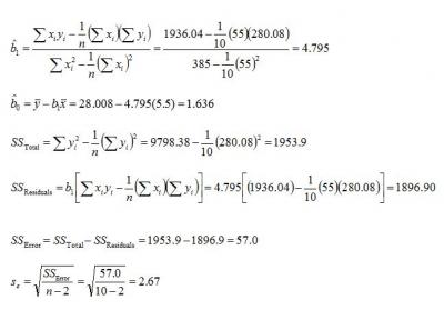
Next, the analyst calculates the value of the response variable, ŷ0, at the desired value of the predictor variable, x. In this case the desired predictor value is 5. ŷ0 = b̂1x + b̂0 = 4.795(5) + 1.636 = 25.61
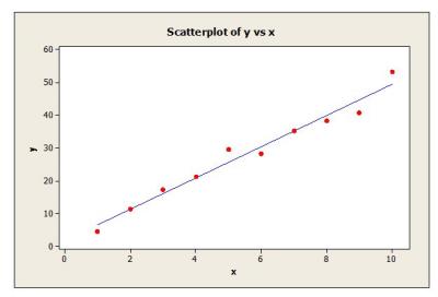
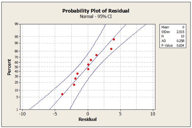
Now, before computing the prediction interval, it would be wise for the analyst to plot the raw data along with the predicted response defined by ŷ0 = b̂1x + b̂0 on a scatter plot to verify the linear relationship. If the data is in fact linear, the data should track closely along the trend line with about half the points above and half the points below (see Figure 3). Data that does not track closely about the trend line indicates that the linear relationship is weak or the relationship is non-linear and some other model is required to obtain an adequate fit. In this case calculation of a prediction interval should not be attempted until a more adequate model is found. Also, if the relationship is strongly linear, a normal probability plot of the residuals should yield a P-value much greater than the chosen significance level (a significance level of 0.05 is typical). Residuals can be easily calculated by subtracting the actual response values from the predicted values and preparing a normal probability of the residual values (see Figure 4).
After establishing the linear relationship between the predictor and response variables and checking the assumption that the residuals are normally distributed, the analyst is ready to compute the prediction interval. The analyst starts by first finding the value for the student’s t distribution equating to a 95% confidence level (i.e., a=0.05). Since the analyst is interested in a two-sided interval, a must be divided by 2. The correct value for t in this instance given that a/2=0.025 and n-2 = 8 is 2.306.
ta/2,n-2 = t0.05/2,10-2 = 2.306With the correct value for ta/2,n-2 in hand, the analyst calculates the interval using Eqn. 6 and the predictor value of 5.
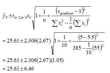
Figure 5 shows the scatter plot from Figure 3 with the calculated prediction interval upper and lower bounds added.
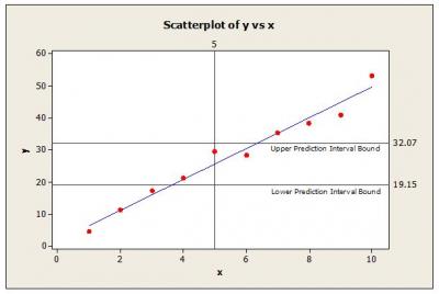
Thus, the interval expected to contain the predicted value for y at x=5 with 95% confidence is 19.15 – 32.07. This procedure must be repeated for other values of x because the variation associated with the estimated parameters may not be constant throughout the predictor range. For instance, the prediction intervals calculated may be smaller at lower values for x and larger for higher values of x.
This method for calculating a prediction interval for linear-regressed data does not work for non-linear relationships. These cases require transformation of the data to emulate a linear relationship or application of other statistical distributions to model the data. These methods are available in most statistical software packages, but explanation of these methods is beyond the scope of this article.
Prediction intervals provide a means for quantifying the uncertainty of a single future observation from a population provided the underlying distribution is normal. Prediction intervals can be created for normally distributed data, but are best suited for quantifying the uncertainty associated with a predicted response in linear regression statistics. Because prediction intervals are concerned with the individual observations in a population as well as the parameter estimates, prediction intervals will necessarily be wider than a confidence interval calculated for the same data set. For the same reason, prediction intervals are also more susceptible to the assumption of normality than are confidence intervals.
In the Part-III of this series we will examine an interval to cover a specified proportion of the population with a given confidence. This type of interval is called a Tolerance Interval and is especially useful when the goal is to demonstrate the capability of a process to meet specified performance requirements such as specification limits associated with a product critical quality characteristic.
Statistical and prediction intervals can be powerful tools for analyzing and quantifying data for your product. Our experts can provide critical consulting services throughout your product lifecycle that will help you to successfully execute projects and bring them to market, while maintaining quality and compliance with applicable regulations and industry standards.
To get started, we invite you to get in touch with our expert consultants or learn more about our Life Science Consulting services. See how ProPharma can help ensure regulatory and development success throughout your product lifecycle!
NIST/SEMATECH e-Handbook of Statistical Methods, http://www.itl.nist.gov/div898/handbook/index.htm Wadsworth, Harrison M. (1990). Handbook of Statistical Methods for Engineers and Scientists. New York, New York: McGraw-Hill, Inc.
Preston, Scott. (2000). Teaching Prediction Intervals. Journal of Statistics Education v.8, n.3
Learn more about ProPharma's Process Validation services. Contact us to get in touch with Fred and our other subject matter experts for a customized Process Validation solution.
TAGS: Statistical Intervals Confidence Interval Process Validation Life Science Consulting
January 16, 2014
We saw in Part 1 of this series how a confidence interval can be calculated to define a range within which the true value of a statistical parameter such as a mean or standard deviation is likely to...

July 10, 2013
Statistical intervals are staples of the quality and validation practitioner’s statistical tool box. Statistical intervals can manifest as plus-or-minus limits on test data, represent a margin of...
May 7, 2012
In a recent FDA Drug Safety Communication, the Agency announced that the Celexa (citalopram hydrobromide) label now has revised dosing recommendations based on evaluations of post-marketing reports...